Example

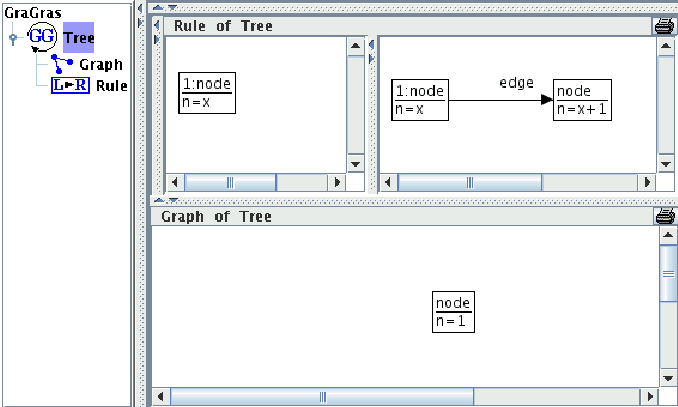
We demonstrate the new layout algorithm by a tree evolution example. An initial tree and a rule to create a new leaf we can see in Fig. 12.

Figure 12: Initial tree graph.

The option settings for this example are shown in Fig. 13 and the table with edge layout patterns is shown in Fig. 14. The layout patterns for this graph grammar forces every child node being placed below its parent node with similar length of edges.

Figure 13: Options of the graph layouter.

Figure 14: Edge Pattern Table.

The Figures 15, 16 and 17 presents the evolution of the tree. We only show the graphs 9, 15 and 24 of the corresponding sequence.

Figure 15: Tree Generation: Graph 9.

Figure 16: Tree Generation: Graph 15.

Figure 17: Tree Generation: Graph 24.

The quality metrics of this tree layout are shown in Figure 18.

Figure 18: The quality metrics of the tree layout.

As we can see, the graph transformation sequence presented consists of 24 graphs.

Columns A, B, and C describe some statistical data. Column A holds the graph position in the sequence which can be described as graph age. Columns B and C hold the number of nodes and edges, respectively. Undesired effects for a single layout are described in columns D, E, F and for the mental distance in columns G, H, the conclusions follow in columns I, J, K. The semantics of table entries is described in more detail below.

These metrics are weighted according to the Offline Graph Drawing Problem which describes the following trade-off for a given graph sequence $G_0 ... G_n$ and their corresponding layouts $L_0 ... L_n$:

• The quality $\rho_{L_{i}}$ of every single layout $L_{i}$ should be as optimal as possible.

• The mental distance $\delta_{L_{i},L_{i+1}}$ from one layout $L_{i}$ to its successor layout $L_{i+1}$ should be small.

• The resulting quality Q of the whole sequence results in the sum of every $\rho_{L_{i}}$ minus every $\delta_{L_{i},L_{i+1}}$,
  

  $$Q_{L_{0} .. L_{n}} = \sum_{i=0}^{n} \rho_{L_{i}} - \sum_{i=1}^{n} \delta_{L_{i-1},L_{i}}$$ (4)

  
  

There are several approaches to measure $\rho$ (the single graph layout quality) and $\delta$ (the mental distance between two graphs).

For the evolutionary layout algorithm we present a specific definition for $\rho$ and $\delta$ which is shown below. We use the table with metrics of the tree evolution example. In this table $d\_single$ stays for $\rho$, $d\_mental$ for $\delta$ and $d\_layout$ for the resulting quality.

1. Weighting of single layout quality $d\_single$:
   A node overlapping (D) is worse than a node-edge-overlapping (E) which is itself worse than a edge crossing (F). In an ideal layout, overlapping nodes would not occur, but they cannot always be prevented, given a large number of edges with strong coupling. Every overlapping must be seen in relation to the number of elements:
   

   $$d\_single = (\frac{B}{D + 1} + \frac{(B + C)}{E + 1} + \frac{C}{F + 1})$$ (5)

   
   

2. Weighting of mental distance $d\_mental$
   A movement of elements must be seen in relation to its number:
   

   $$d\_mental = \frac{H}{B} + \frac{G}{C}$$ (6)

   
   

3. Resulting layout quality $d\_layout$:
   
   

   $$d\_layout = d\_single - d\_mental$$ (7)

   
   
   To summarize these effects, the quality of a single layout is given in column I, in column J the mental distance to the previous layout and in column K the resulting quality as described by (4) are shown.
   

If the start layout is easy to understand and the following layout differences are small, then a user can keep track even if the graph (and its layout) gets more and more complicated.

Back to our example, we take a look at the table in Fig. 18 in more detail.

As we can see, node-node overlappings do not occur during the whole transformation sequence. A small number of node-edge overlappings and edge-edge crossings do occur. For the first 11 layouts, the edge and nodes movements are rather unstable. This implies quite different single, mental and resulting layout quality, especially for the first 4 layouts. But the larger the graph grows, the better the layout quality becomes.

So we can summarize that the disturbance is small given the number of node and edges and their crossings. The algorithm is able to turn back to a better layout. The edge type pattern for the tree layout is applied successful.

Last but not least, we compare the graph layout of the tree example shown above with the graph layout of the same tree example but without using layout patterns (see Fig. 19)

Figure 19: Tree graph that is generated without layout patterns.

and finally, with the graph layout of the same tree example but without using the evolutionary layout algorithm (see Fig. 20).

Figure 20: Tree graph that is generated without evolutionary layout.

The graph in Fig. 19 looks like more a spider web due to its radial layout and in Fig. 20 like a brickwork but not like a tree.

As conclusion we can say that our algorithm produces readable layouts and can be used for a graph transformation sequence as well as for incomplete sequences of class models or other graph-like diagrams which are converted to the AGG graph format. Future work concerns extending and improving layout patterns for graph transformation sequences.

The ''Evolutionary Layout of Graph Transformation Sequences'' is a common work of SWT and TFS at TU Berlin.

More details are described in:

• D.Graf, "Evolutionaeres Layout von Graphsequenzen unter Nutzung von anwendungsspezifischen Vorwissen", Master Thesis, TU Berlin, 2006.

  (http://tfs.cs.tu-berlin.de/agg/Diplomarbeiten/ELofGTS-diplomDGraf.pdf.zip).

• "Evolutionary Layout of Graph Transformatio Sequences" by Susanne Jucknath-John and Dennis Graf and Gabriele Taentzer, ISSN to be provided, 2006.